
- Key Takeaways
- Core Inputs of Aggregate Production
- Foundational Macroeconomic Models
- Long-Term Growth Dynamics
- Measuring Modern Structural Shifts
- Critical Theoretical Limitations
- Strategic Policy Recommendations
- Conclusion
- Frequently Asked Questions
- What are the main inputs in aggregate production?
- How do macroeconomic models explain aggregate output?
- What drives long-term economic growth?
- How are structural shifts in production measured?
- What are key theoretical limitations in aggregate production models?
- Which policies best support aggregate production growth?
- How can policymakers measure policy impact on output quickly?
Key Takeaways
- Aggregate production relies on labor, capital, and natural resources in concert, and fortifying digital infrastructure and resource management enhances output and sustainability. Focus on capacity planning and technology to stabilize supply.
- Workforce skills and training directly increase productivity at industries, so spend on education and upskilling initiatives to help increase aggregate production and minimize production frictions.
- Boosting capital per worker with state-of-the-art machinery and facility enhancements drives long-run output. Strike a balance between capital deepening, labor, and costs to prevent diminishing returns.
- Total factor productivity gains from innovation, process improvement, and digital tools are the heart of GDP growth, so track productivity tendencies and back R&D and automation to anticipate and grow output.
- Save natural capital by optimizing resource distribution, recycling crushed concrete and extracting resources sustainably to postpone raw material shortages and minimize risk to the environment.
- Be skeptical of aggregate production models, like Cobb-Douglas and constant elasticity, given capital measurement and intangible omissions. Augment their models with information on intangibles, digital adoption, and structural changes when making policy or investment decisions.
Aggregate production is when they make crushed stone, sand, and gravel for construction purposes. It includes quarrying, crushing, screening, and washing to satisfy size and quality regulations.
Producers control hardness, particle shape, and grading to suit concrete and asphalt specifications. Outputs impact material costs, structural performance, and carbon due to transport and processing.
The subsequent chapters discuss production phases, quality controls, and optimization alternatives for city and regional-scale projects.
Core Inputs of Aggregate Production
Aggregate production relies on some core inputs that collectively establish the scale and efficiency of production. Core inputs of aggregate production include labor, capital, and natural resources. Their abundance and quality in society define total output, while digital infrastructure and resource planning optimize and sustain supply.
A common specification for the aggregate production function is output as a function of labor and capital, which is weakly increasing, weakly concave, continuous, and commonly assumed to have constant returns to scale. Cobb-Douglas is a popular functional form for capturing those relationships.
1. Labor Quality
Worker skills, education and training increase individual and firm productivity in mining, quarrying and processing activities. Skilled workers make fewer comminution and sieving errors, perform equipment changeovers faster, are safer, and thereby increase aggregate output per worker.
Manufacturing utilizes more routine, assembly-oriented skills. Construction requires multi-skill crews and in-person expertise. Mining and quarrying demand technical expertise for blasting, dredging, and in-stream extraction. Changes in labor quality thus move productivity between sectors.
Labor compensation and hours worked connect directly to output. Higher pay can attract better-trained workers and reduce turnover, which supports steady production. Overtime can increase short-run production but reduce long-run productivity due to exhaustion and injuries.
Spending on training, apprenticeship, and certification for aggregate production raises efficiency and reduces downtime.
2. Capital Deepening
Capital deepening is more or better capital per worker to push output higher. Think automated crushers, GPS guided loaders, upgraded washing plants and enhanced storage and handling of graded aggregates. Capital deepening reduces comminution cycle times and enhances size classification.
Capital investment increases aggregate supply and sustains long-run growth by permitting increased throughput and reduced unit costs. It shifts cost structure: more capital can lower variable labor costs but raise fixed costs and capital recovery needs.
Consider payback periods and capacity when designing equipment upgrades.
3. Total Factor Productivity
TFP, in essence, captures how well labor and capital combine. Innovation in process flow, improved maintenance schedules, and process automation increase TFP by minimizing leakage and downtime during sieving, stockpiling, and transport.
Rising TFP raises GDP without necessarily raising inputs by the same proportion. Tracking TFP trends helps forecast aggregate output changes.
Apply productivity figures linked to throughput per hour, yield after comminution, and water consumption per tonne.
4. Natural Capital
Natural capital covers minerals, soil, and water, as well as geological resources for sand, gravel, and crushed stone. Quarrying and mining provide these from dry pit to in-stream sand dredging and feature different water consumption.
Surface mine — finite resources sustainability challenges managing reserves, zoning, rehabilitation. Repurpose broken concrete and mill sand to conserve natural capital and reduce stress on waterways.
5. Digital Infrastructure
Digital tools make possible improved planning, forecasting, and automation throughout the aggregate chain. Connected sensors on crushers, real-time inventory systems, and data analytics optimize scheduling, minimize stockouts, and eliminate oversupply.
Digital adoption is helping to manage demand variability and optimize water and energy use. Putting these solutions in place cuts costs and increases reliability, enabling a more robust and efficient aggregate supply.

Foundational Macroeconomic Models
Foundational macroeconomic models capture aggregate production by connecting inputs, prices, and policy to overall output. They demonstrate how capital, labor, and technology aggregate into supply and how demand, price levels, and policy moves transform output in the short and long run.
These encompass production functions that tie inputs to output and system-level frameworks such as AD-AS and IS-LM that situate production in a marketplace.
Cobb-Douglas Formulation
This is similar to foundational macroeconomic models of output where Y equals A multiplied by K raised to the power of α and multiplied by L raised to the power of β. In this equation, K represents capital, L represents labor, and A stands for total factor productivity.
The variables α and β are output elasticities; a 1% rise in K raises Y by roughly α percent, holding other terms fixed. The same applies for L and β. When α plus β equals 1, the function has constant returns to scale. Doubling K and L doubles Y, which serves as a useful benchmark for balanced growth.
The Cobb-Douglas form links to macro issues. A captures technology shocks that shift the AD-AS equilibrium by changing potential supply. Changes in K and L feed into the SRAS through capacity and utilization.
Industry examples: in manufacturing, α may be larger, reflecting capital intensity. In services, β could be higher, indicating labor intensity. Cross-sector estimation reveals how policy that impacts investment or labor supply translates to output.
Employ Cobb-Douglas for short-run supply reactions. A good productivity shock increases A, moving SRAS right and alleviating price pressure at a given AD. Monetary or fiscal stimulus shifts AD.
Along with a given Cobb-Douglas supply, you can map out output, unemployment, and price shifts. This connects micro elasticity to macro dynamics.
Constant Elasticity
CES or constant elasticity of substitution explains how easily capital and labor substitute for one another. CES nests Cobb-Douglas as a special case when elasticity equals one. Elasticity greater than one implies inputs are easy to substitute, while less than one makes them harder to replace.
Large substitution elasticities provide firms flexibility when relative factor prices change, smoothing output when wages or capital costs move. Low elasticity translates into inflexible input mixes.
Shocks to capital or labor generate larger output oscillations and magnify short-run SRAS fluctuations. CES therefore changes the way supply reacts to demand and policy shifts.
Unlike Cobb-Douglas, CES adjusts well to input price ratios. It can demonstrate, for instance, how automation, with capital costs falling, will increase output more when substitution is higher.
The IS-LM framework and AD-AS story take these production forms and use them to map goods-market equilibrium to money-market conditions and to illustrate policy effects.
|
Substitution rate |
Typical outcome on output |
|---|---|
|
Low (<1) |
Output sensitive to specific input shocks |
|
Medium (approximately 1) |
Cobb-Douglas type balanced response |
|
High (>1) |
Firms move inputs, smoothing output variations |
Long-Term Growth Dynamics
Long term growth dynamics takes a look at how persistent increments in aggregate output lead to general economic growth over various time scales. Growth is driven by shifts in aggregate supply, but the process shows low persistence. Growth rates often have weak inter-temporal correlations, which makes long-term forecasting difficult and requires careful attention to underlying drivers rather than past trends.
Technological Progress
Technological advancement increases the amount an economy can produce with given inputs. These can be advances in production technology, like better machine tools, modular construction techniques, or factory floor digital twins. They increase total factor productivity and move the aggregate production frontier outward.
Automation and digitalization reduce unit costs and increase throughput by replacing repetitive work, allowing workers to concentrate on value-added tasks. Process innovation, such as lean production or continuous-flow manufacturing, cuts waste and cycle time, increasing both capacity and demand responsiveness.
Firms that invest in R&D and in capital equipment experience measurable productivity gains, and the relationship between firms’ R&D intensity and output growth is well documented in manufacturing and construction industries. Capital investment funds new technology and capital deepening, which means more machines per worker, increases labor productivity.
Help firms internalize the long-term growth dynamics of emerging technologies by making investment appraisal consistent with multi-year productivity gains and by using pilots to reduce adoption risk. These can range from sensor-driven approaches to minimize downtime in factories to BIM in construction to reduce rework.
Diminishing Marginal Returns
The law of diminishing marginal returns says that if you add more of one input while holding other inputs constant, the output gains will get smaller and smaller. At the aggregate level, if you add labor to a fixed stock of machinery or add more of the same machines without increasingly more skilled operators, you will get diminishing marginal output.
An example is hiring 10% more workers in a plant with fixed tooling. This may raise output substantially at first, but further hires produce less additional output unless machinery or training increases. Over-investing in one input, such as a big capital purchase without accompanying labor skills or spare parts, can lead to idle assets and diminished returns.
Watch the marginal product of each input to steer investment decisions and rebalance resource allocation. Use these short-run indicators, such as production per worker, machine utilization, and short-term forecast errors in output, to help detect when marginal returns fall.
Studies demonstrate that growth rates have no strong persistence and short-term investment spikes, lasting from one quarter to one year, can signal forthcoming expansion. However, aggregate investment measures forecast lower one-year ahead REIT excess returns.
Strategies for aggregate production planning to meet future demand:
- Align investment timing with demand signals and lead times.
- Diversify input upgrades: balance capital, labor training, and maintenance.
- Use scenario-based capacity planning and stress tests.
- Track marginal product metrics and short-term forecast errors.
- Invest in modular, scalable technologies for flexibility.
Measuring Modern Structural Shifts
Capturing how aggregate output shifts needs a precise frame connecting what companies make, who labors, and what machines they deploy. Start by mapping shifts in technology, labor markets, and capital investment to observable series: output by sector, hours worked, capital stocks, and multifactor productivity.
Use firm- and industry-level data to mitigate noise from firm churn and capture the large-scale reallocation of outputs and inputs across producers. Shift-share and decomposition tools connect these micro shifts to macro results.
Follow changes in the aggregate production structure as a result of technology, labor markets, and capital investment. It measured adoption of new technology as changes in capital composition and productivity per worker.
Characterize labor-market change with respect to employment shares, skill composition, and rates of job reallocation. Record capital investment by type, which includes physical machinery, software, and infrastructure, and layer age and utilization rates.
Connect these series to output growth that can show whether higher output is coming from more inputs, improved use of inputs, or from shifting to higher productivity firms.
About: Quantifying Contemporary Structural Changes. Calculate labor and multifactor productivity at firm and industry levels. Then perform shift-share analysis to break down aggregate growth into within-industry productivity gains, between-industry reallocation, and input growth.
Shift-share analysis gives us a handy method to explore how aggregate growth is mechanically connected to differential growth of labor productivity and the reallocation of labor between industries. Decomposition analysis can at best uncover the direct contributions of structural shifts at the industry level to aggregate growth performance.
Supplement it with firm-level microdata to catch indirect effects. Measure modern structural shifts. Leverage long-run series to demonstrate that structural changes across sectors have dragged trend GDP growth down by roughly 2 percentage points since the early 1950s.
Search for time-varying elasticities of aggregates with respect to aggregate shocks because one important implication is that these elasticities shift as the industrial mix evolves. Historical comparison shows how demand-induced sectoral shifts, heavy technology, and negligible foreign trade all underline the significance of structural changes.
- Significant structural shifts in point form:
- Fast adoption of digital and automation technologies is changing capital composition.
- Increasing service and manufacturing decline in many economies.
- Skill-biased labor demand is fueling wage and employment dispersion.
- High-powered horizontal and vertical spillovers exist.
- Capital deepening in knowledge-intensive sectors is pushing up multifactor productivity.
- Demand shifts are fueling sectoral growth regardless of trade flows.
The micro process is noisy. Business and worker churning is constant as agents search for better matches, and this makes measured growth volatile even when the long-run trend shifts slowly. Industrial structure still shapes macro development.
Critical Theoretical Limitations
Aggregate production functions attempt to capture such input/output mapping at an economy-wide level, yet they gloss over these complexities. They squeeze firms, sectors, and technologies into a handful of parameters, which obscures variation in know-how, practices, and organizational environments.
About: Accounting Critique. The accounting critique contends that fitted aggregate functions typically capture accounting identities and value shares rather than causal production relationships, so statistical fit provides no evidence of structural validity.
Cambridge Capital Controversy
The Cambridge debate raises the question of how to measure capital and whether capital can be treated as a single, well-defined magnitude at all in aggregate models. On one side, they demonstrate that heterogeneous capital goods have no inherent common unit other than price weighting, which depends on income distribution, thereby breaking circularity and sinking the marginal productivity story.
Aggregation of heterogeneous capital goods into a single K is troublesome. Machines, buildings, software, and financial assets vary in durability, vintage, and productivity. A single index is highly susceptible to measurement choices and price signals.
The challenge of measuring finance-sector output exacerbates this issue because financial assets frequently arrive in accounts via valuations rather than physical flows. Implications ensue for reading output elasticities and returns to scale. If capital is mismeasured, then estimated elasticities can reflect accounting choices, not technology, and constant returns to scale assumptions are suspect.
Even empirical Cobb-Douglas fits, while they look neat because they use value data, conceal these conceptual voids. At a critical theoretical level, modelers must specify what capital is, specify aggregation rules, and test sensitivity to alternative measures and distributional assumptions.

Intangible Asset Omission
Standard production functions typically leave out intangible assets like knowledge, organizational capital, and brand equity. This omission biases measured total factor productivity downward and shifts unexplained residuals to a mysterious “technology” term, which conceals important drivers of growth.
Leaving intangibles out underestimates output and productivity. Software, patents, data, or strong customer ties make firms that rely on them produce more value with similar tangible inputs. Aggregate functions that omit these items attribute output to unexplained residuals or mismeasure returns to labor and capital.
Updating models to incorporate intangible inputs enhances both explanatory and policy power. That needs improved data, novel means of measurement and functional forms nimble enough to accommodate nonrival, scalable assets and network effects.
Practical policy must use caution. Applying simple theoretical models to tax, subsidy, or industrial policy risks misdiagnosis if intangibles or finance-sector measurement issues are ignored.
Examples of intangible assets:
- Intellectual property (patents, copyrights)
- Brand value and reputation
- Software and proprietary algorithms
- Organizational capital and processes
- Customer relationships and data
- Human capital in tacit skills
Strategic Policy Recommendations
Strategic policy recommendations direct decisions on how much to produce, whom to hire, and how much inventory to carry to optimize resource usage given customer demand and profit goals. Aggregate planning, which covers three to eighteen months, provides a unified picture that connects demand, production, procurement, logistics, and capacity.
Policies should help firms set capacity targets, match units produced to customer demand, and weigh the five core costs: regular time, overtime, subcontracting, inventory holding, and back-ordering.
Invest in education, workforce training, and digital infrastructure to increase aggregate output. Training increases worker skill, enabling firms to use more flexible staffing and cut overtime and subcontracting costs. Digital tools that enhance demand prediction reduce inventory overhead and back-order expenses by aligning supply and demand more closely.
Concrete measures include subsidy programs for vocational training, tax credits for on-the-job upskilling, and grants for cloud-based planning systems that incorporate metric data and common currency inputs for global supply chains.
Back research and innovation to raise total factor productivity and accelerate technological advances. Public process research funding, joint industry-university labs, and fast-track approval for pilot production lines allow firms to trial automation and process changes without large upfront risk.
Policies that favor open standards and shared data platforms enable smaller firms to tap into advanced planning tools. Examples include co-funded pilot projects for smart batching in concrete or recycled aggregate sorting that reduce waste and lower regular time costs.
Incentivize sustainability and recycling in aggregate industries. Tax incentives for recycled-content use, subsidies for material recovery facilities, and minimum recycled-content mandates all move demand in the direction of circular inputs and reduce raw material supply risk.
This reduces procurement volatility and long-term expenses related to resource scarcity. Provide explicit subsidies for low-energy crushing and washing equipment and for water reuse in metric tons saved per year to incentivize actual, tangible progress.
Promote public-private cooperation to adjust total output with sustainable growth objectives. Form sector councils to establish shared forecast scenarios, cost standard rates and hybrid strategies that combine level, chase and outsourcing approaches to accommodate complex demand.
Leverage joint scenario planning to establish capacity buffers and make decisions on when to utilize overtime, subcontracting or inventory build. Policies should mandate cost transparency for the five cost categories and incentivize best-practice toolkits for demand forecasting, capacity calculation and cost trade-off analysis.
Conclusion
The article stitches the pieces together into a nice perspective on aggregate production. It demonstrates how inputs, models, and data connect to growth and policy. Simple models provide fast sanity checks. Rich models provide deeper tests, and measurement instruments discover actual changes in technology and need. Bounds in principle indicate holes in observations and required model corrections. Policy actions focus on improved investment, skills, and market reforms to boost production and employment.
An example is that a city boosts public transit, firms cut commute time, labor supply rises, and output climbs. Another example is that a skills voucher helps young workers join high-productivity firms and raises firm-level output.
Experiment with a single variation that suits your situation. Follow basic measures such as time spent, capital utilized, and aggregate production. Use them to measure impact.
Frequently Asked Questions
What are the main inputs in aggregate production?
Aggregate production is dependent on labor, capital (both physical and human), natural resources, and technology. These inputs aggregate in production functions to determine output and productivity for an economy.
How do macroeconomic models explain aggregate output?
Fundamental models, such as the Solow or Keynesian models, connect output to inputs, savings, investment, and demand. They exhibit short run demand phenomena and long run supply driven growth trajectories.
What drives long-term economic growth?
Long-run growth results from productivity growth, technological innovation, human capital accumulation, and wise investment. Institutional quality and stable policy matter for enduring growth.
How are structural shifts in production measured?
Economists employ sectoral shares, productivity differentials, employment patterns, and value-added statistics to monitor this transition away from agriculture and toward manufacturing and services.
What are key theoretical limitations in aggregate production models?
Models typically abstract from heterogeneity, distributional effects, and assume efficient markets. This restricts real-world forecasting, particularly in the case of shocks or structural shifts.
Which policies best support aggregate production growth?
Policies that make education, R&D, infrastructure and business regulation better raise productivity. Sound macroeconomic policy and focused investment allow for continued production growth.
How can policymakers measure policy impact on output quickly?
Instead, rely on high-frequency indicators such as industrial production, employment, and investment surveys. Pair these with model-based nowcasts for up-to-date evaluation and adjustment.